
Building portfolio seismic fragility analysis: incorporating building-to-building variability to carry out seismic fragility analysis for reinforced concrete buildings in a city

Abstract
Predicting how future earthquakes will affect structural performance in a particular region is a challenge due to the unpredictable nature of earthquakes and inherent uncertainties in construction materials and the geometry of structures. This study considers building-to-building variabilities as inputs in an existing Response Surface Methodology (RSM) that are based on the Design of Experiment (DoE) technique to quickly determine the structural fragility of a region. As it is impractical to analyse each individual structure in a region in detail, this study addresses the issue by collecting a set of building parameters and using screening design to evaluate the most significant building parameters in the overall seismic performance. Instead of performing building-to-building analyses, the propagation of uncertainty in building-to-building variability can now be performed using a polynomial response surface metamodel. The metamodel is a function of the response of the building, and a set of significant parameters. This study aims to obtain the fragility of a collection of buildings with the help of the existing RSM by considering variability in structural parameters that can represent the overall structural geometric and material properties within a region. A case study is conducted for the collection of reinforced concrete (RC) buildings in the city of Silchar, located in Northeast India, which is one of the most seismically active regions of the country. The fragility curve developed with significant building parameters from RSM has been compared with that of the conventional method using Incremental Dynamic Analysis (IDA), and the match of the result confirms the accuracy of fragility assessment using RSM.
Keywords
INTRODUCTION
The conditional probability of exceeding specific limit states at a certain level of seismic intensity is known as seismic fragility[1]. A fragility curve, obtained by integrating the probability of failure across various seismic intensity levels, shows the likelihood of a building sustaining damage as the seismic hazard increases. Since earthquakes are complicated natural events and no two earthquakes are alike, it is difficult to predict how well a building would perform in the event of a future earthquake[2]. As the construction material qualities and geometrical configurations differ from building to building within an area, the building itself is another source of uncertainty. Generic fragility curves are usually employed to quantify damage assessment of buildings which fall under similar types[3]. However, fragility curves may vary among buildings in the same classification due to variability in geometric configurations, material properties, age of the building, etc. Therefore, fragility evaluation for a collection of buildings is required for a more accurate damage estimation in the region. Property owners, insurance firms, capital lending institutions, and local government agencies are particularly interested in quantifying the potential effects of earthquakes on a collection of buildings in seismically-prone locations. Each such stakeholder is likely to have a distinct perspective and needs. For instance, insurance firms and corporate risk managers are often interested in the behaviour of a collection of structures scattered over an area. In this situation, the Federal Emergency Management Agency (FEMA) guidelines and its practical implementation in a performance-based assessment approach, e.g., the Performance-Based Earthquake Engineering (PBEE) framework[4] over building-specific fragility models would be more appropriate and should be the preferred choice. Although performing nonlinear time history analyses (NLTHA) can yield building-specific fragility curves, the simulation requires enough time for each building. Therefore, taking building-to-building variability into account for fragility evaluation becomes unfeasible when such simulations are done for a range of buildings.
Seismic fragility analysis (SFA) is not a new method for predicting the probability of damage to a building at various earthquake intensities. Numerous studies on SFA can be found in the literature[5-10]. Analytical fragility curves or damage probability matrices (DPM) are typically used to represent fragility[11,12]. DPM indicate the relationship between ground intensity measure and probability of damage to be discrete, while the analytical fragility curve indicates the same relationship to be continuous. Early studies on fragility[13,14] relied on the capacity spectrum approach with nonlinear static analysis, while more recent studies[1,15-17] use the Incremental Dynamic Analysis (IDA) procedure[18] to obtain the capacity. An extensive review of fragility derivation methodologies can be found in[19,20].
Epistemic uncertainties arising from specific modelling of buildings can be effectively addressed by using numerous statistical models. However, few studies have addressed the seismic fragility modelling by considering building-to-building variability for seismic risk assessment across a portfolio of buildings scattered over an area[11,21-23]. A study conducted a case study on a group of wood-frame houses in Canada to illustrate the current approaches for quantifying risk[24]. The study introduced a concept of building portfolio fragility function (BPFF), which was defined as the probability that a building portfolio, as an aggregated system, fails to achieve prescribed performance objectives given scenario hazards. The function was used to characterise the vulnerability of a building portfolio[25]. To determine the most appropriate analytical fragility curves for each building class and geographic area, an extensive investigation was conducted to examine the procedures and methodologies for evaluating the seismic vulnerability of the existing building stock in Europe. This involved collecting and reviewing numerous analytical fragility curves from the technical literature in depth[26]. For Nepali unreinforced masonry (URM) school typologies, a spectral-based methodology was used to construct fragility curves, which considered both in-plane and out-of-plane damage within a single and simple analytical framework[27].
In recent years, there have been efforts to address the uncertainty in building properties within SFA. One such effort involved the creation of a web-based application that enables users to categorise a specific building stock based on key structural parameters[28]. The authors also described the development of an analytical fragility model that covers the most typical building classes globally. This is achieved through time history analyses conducted on Equivalent Single Degree of Freedom (ESDOF) oscillators. Extensive field surveys were carried out to determine building-to-building variability, and some representative buildings were identified for fragility analysis using time history analyses[29]. However, this simulation technique requires a high computational cost to obtain the desired output. To mitigate the computational demands, researchers discovered the effectiveness of the Response Surface Methodology (RSM), which may substitute complex models with high processing requirements[30]. The nonlinear dynamic response of the structure needed for SFA was explored with an effective Moving Least Square Method (MLSM)-based RSM[31]. By integrating this approach as one of the predictors in the seismic response prediction model and using it as a control variable, it was suggested that it could be used wisely to avoid the need for the repeating of intensity for the full fragility curve development. To account for building-to-building variability in simulation-based seismic risk assessment of a portfolio of buildings, Gaussian process regressions were employed to create flexible and precise metamodels[22]. It is also noteworthy that the simulation-based SFA used the Monte Carlo Simulation (MCS) framework for probabilistic experimentation and Latin Hypercube Sampling (LHS) approach for generating RSM[32].
The present study offers several novel aspects that address the limitations of previous RSM studies. These aspects are highlighted below:
• The variability in parameters across buildings that influence the response is taken into account to depict general building characteristics within a specific region.
• The number of ground motions selection criteria for performing nonlinear time history analysis is based on American Society of Civil Engineers (ASCE) version 7-16 code guidelines rather than arbitrary selection. The ground motions are selected from FEMA P-695, which suggested standardised ground motion records to obtain fragility based on epicentral distance, focal depth, magnitude, attenuation, and slip distribution.
• With the help of the fragility curve developed through RSM for a specific building, the fragility curve of any other arbitrary building can be predicted without calculation, provided that the most significant parameters obtained from the screening design have identical values for both buildings.
The study was conducted at a test site in Silchar, a city in North-Eastern India. Rapid Visual Screening (RVS) and expert opinions have been employed to gather information on building input variables to account for building-to-building variability. The overall methodology involved six-step key points, as described below (see Figure 1):
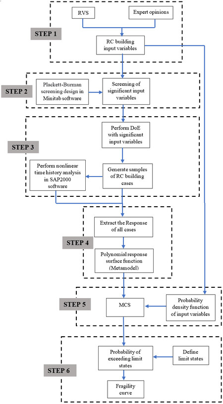
Figure 1. Flow chart of the overall methodology.
1. Data collection of building-to-building variability according to the age of construction.
2. Screening of the collected data to identify the most significant building parameters.
3. The Design of Experiment (DoE) approach is then used to efficiently create building parameter samples, specifying a collection of building model cases. NLTHA are performed on each case.
4. The building parameter samples and the resulting outputs (Inter-Storey Drift (IDR) ratio) are then subjected to least-square regression analysis to form a metamodel in the form of a polynomial response surface function.
5. The metamodel is subjected to MCS by repeatedly computing the responses while randomly choosing values for the input variables based on their assumed probability density.
6. The probability of exceeding limit states for a specific level of intensity measure is calculated by dividing the number of times the computed response exceeds the limit state thresholds by the total number of simulation trials. This process is repeated for various levels of intensity measures to produce the fragility curve.
DESCRIPTION OF THE METHODOLOGY
Step 1: collection of building inventory data
In large-scale fragility studies of a region through an analytical approach, a crucial aspect is the building inventory data, particularly the understanding of the distribution of the attributes that mainly affect seismic fragility. The parameters may include building typology, force-resisting mechanism, construction material, age of the building, building configuration, percentage of reinforcement, ductility, seismic design level, number of stories, and load characteristics.
Macro seismic intensity measures, such as the Medvedev-Sponheuer-Karnik (MSK-64) scale, were first used to collect the building data. Buildings were initially divided into three distinct vulnerability classes, A, B, and C, based on their material and types of load-bearing systems on the MSK-64 scale. The European Macro Seismic Scale (EMS) later adopted the MSK-64 classification system, classifying structures into six categories (from A to F), depending on the type of construction material used and the level of code design[33]. Later, the Hazard United States (HAZUS) methodology proposed classifying the existing building stock into several Model Building Typologies (MBTs) based on structural type, height range, and codal provisions[3].
When developing a building inventory data, different approaches can be followed depending on the data availability and resources. At the regional scale, information coming from remote sensing, satellite imagery, national housing databases, RVS from field surveys and expert judgements are commonly utilised[11]. For the present study, RVS data and expert opinions have been considered to collect the building-to-building variability data, as information from other data sources cannot be extracted for this region. Inventory data can be in the form of 32 MBTs, as proposed by the HAZUS building classification[3]. Each type comes with inherent variability in its geometrical and material properties over a region. The ability of a building to withstand an earthquake is greatly influenced by the seismic design requirements that it complies with. Therefore, the assumption in the present study is that the seismic design requirement corresponds to the construction year of a structure. There are four Indian Standard (IS) codes: IS 1893:1962 (covering the years from 1964-1984), IS 1893:1984 (1984-2002)[34], IS 1893:2002 (2002-2016)[35], and IS 1893:2016 (2016-present)[36]. Pre-1984, building data is almost unavailable; thus, only three codes are considered. Therefore, the “Low-Code” (LC), “Mid-Code” (MC), and “High-Code” (HC) are assigned to buildings with construction years in the intervals of “1984-2002”, “2002-2016”, and “2016-present”, respectively.
Step 2: screening design
When there are multiple variables or input parameters for a building, screening is used to limit the number of variables by selecting the most important ones that have an impact on the seismic performance of the building as a whole. This reduction allows one to focus on the process improvement efforts connected with the few really important factors. Screening designs provide an effective way to consider a large number of variables in a minimum number of experimental runs or trials (i.e., with minimum computation cost). There are mainly two types of screening design, Definitive screening design and Plackett-Burman screening design. A definitive screening design can be used to study the effects of main effects, two-factor interactions, and quadratic effects, whereas the Plackett-Burman screening design enables one to study the main effects only. For example, if there are ten variables, a definitive screening design helps to identify the significance of all the ten variables as an individual and the interaction of any variable. Additionally, the Plackett-Burman design does not consider the interaction effect. A detailed discussion of this concept can be found in the literature[37-39].
The present study incorporates the Plackett-Burman screening design as its primary purpose is to identify significant variables rather than the interaction effect, which is assumed to be of lesser importance. In this design, only two levels of the variables (lower bound denoted by -1 and upper bound by +1) are used to construct a sample of various building cases. For example, if there are four variables, a, b, c, and d, the first sample case assigned -1 to a and b and +1 to c and d, then the first case of the building will be constructed by using the lower bound value of a and b and upper bound value of c and d. The response is then evaluated for all the cases by performing computational analysis. To determine the impact of each input variable on the output, a first-order regression model is to be created, as shown in Equation (1)[2].
where y = response and βi (i = 1 to 4) are coefficient estimates. Minitab statistical software (Minitab 19.2020.1) has been used in the present study to carry out the screening design. The statistical validation of the regression model is to be checked for adequacy and reliability. The output of the screening design is presented in the form of bar columns, indicating the decreasing order of significance[40]. The variable with the longest bar has the greatest impact on the output. Even a slight change in the input value of the significant variable has a substantial effect on the calculation of the output, assuming all other input variables remain constant.
Step 3: design of experiment
A complex computational analysis must be performed to obtain the response because the precise relationship between a response and a set of input variables is implicit. The alternative approach is to develop a metamodel (also known as RSM), which is a statistical approximation of the relationship. This approach estimates the response as a function of the input variables, thereby making the computation easier. The DoE method provides the necessary framework for this crucial stage of RSM[40]. The responses must be estimated at an efficient set of experimental sampling points, as defined by the DoE. Each sampling point indicates a specific building model case. The DoE creates a variety of combinations at which the outputs are computed while taking into account a variety of input variable ranges. Care must be taken while selecting meaningful ranges for the input variables. The ranges must be large enough to encompass all feasible parameter spaces while being constrained enough to allow for easy matching of the response surfaces by regression to the actual response. Many types of DoEs can be used for this purpose, such as the Full Factorial Design (FFD), Central Composite Design (CCD), Box-Behnken design, the Space-Filling design, and Taguchi’s orthogonal arrays[41]. However, FFD and CCD are the most frequently used[40]. In the present study, CCD has been used as it requires fewer sampling points while keeping respectable prediction accuracy. A detailed discussion regarding the DOE techniques can be found in[38,40]. Minitab statistical software has been used in the present study to generate sampling points with the help of CCD.
Response simulation by computational analysis
To obtain accurate damage statistics for structures, repetitive nonlinear dynamic analyses, i.e., NLTHA, need to be done. Since three codal provisions have been selected for the evaluation of the response of buildings, three different sets of sampling points are developed by using CCD, according to the building inventory data collected for the three codal provisions.
Building inventory data considers structural parameter uncertainty. Earthquake ground motion records are incorporated into the NLTHA on each sampling point or building model case to account for uncertainty in seismic loading, as the overall seismic performance of the building depends on both structural parameters and the intensity of the earthquake it is subjected to. Therefore, to define building-to-building variability, earthquake intensity measure or Peak Ground Acceleration (PGA) is added as another variable. Sampling points are then generated with the help of CCD. PGA is selected because it is one of the most prominent earthquake intensity parameters for the estimation of damage states and derivation of fragility curves[1,42-45].
A collection of earthquake records is used to account for the uncertainty in seismic inputs. Historical seismic events should be used to derive the ground motions in a suite with randomly varying parameters, such as the epicentral distance, focal depth, magnitude, attenuation, and slip distribution[46]. Hence, to consider the variability in seismic inputs, earthquake records are to be selected. FEMA, 2009[47] suggested 22 robust far-field ground motions that were selected based on large magnitude events, source type, site conditions, source-to-site distance, and the number of records per event. These records are useful for the collapse assessment of buildings. However, according to the American Society of Civil Engineers (ASCE) guidelines[48], 11 earthquake records are sufficient to obtain a reliable estimate of seismic responses, considering record-to-record variability. Therefore, the present study considered 11 earthquake records from the suggested 22 ground motions by FEMA, 2009, which are shown in Table 1. These 11 records are considered based on the magnitude range of Mw (6.5-7.6) and PGA range of 0.24-0.82 g.
Summary of ground motion records considered
| S.No. | Magnitude (Mw) | Year | Location | Recorded PGA (g) |
| 1 | 6.7 | 1994 | Northridge | 0.48 |
| 2 | 7.1 | 1999 | Duzce | 0.82 |
| 3 | 7.6 | 1999 | Chi-Chi | 0.51 |
| 4 | 6.5 | 1979 | Imperial Valley | 0.38 |
| 5 | 6.9 | 1995 | Kobe | 0.24 |
| 6 | 7.5 | 1999 | Kocaeli | 0.36 |
| 7 | 7.3 | 1992 | Landers | 0.24 |
| 8 | 6.9 | 1989 | Loma Prieta | 0.56 |
| 9 | 7.4 | 1990 | Manjil | 0.51 |
| 10 | 6.5 | 1987 | Superstition Hills | 0.36 |
| 11 | 7 | 1992 | Cape Mendocino | 0.55 |
Now, each sampling point defines a building model case which is subjected to the 11 ground motions, scaled to a particular earthquake intensity measure (PGA, herein). Models for predicting response at specific levels of PGA are developed by analysing the response surface at various PGA values. The PGA variable is used in the same manner as other input variables when developing a response surface model. Definitions must be made for the lower, centre, and upper bound of PGA. In this study, the values of 0.1 g and 0.6 g denote the lower and upper bound, respectively, for PGA, while the centre value is assigned as 0.35 g. The upper bound of 0.6 g is based on the hazard level for Maximum Considered Earthquake (MCE) obtained from a hazard analysis study conducted for Silchar City[49,50]. There are three sets of 11 scaled ground motions. For a lower bound case, the first batch of accelerograms has PGA values scaled to 0.1 g. The centre (0.35 g) and upper bound (0.6 g) are used for the second and third batches, respectively.
Next, NLTHA is performed on a building model defined by the DoE step. The buildings are designed according to the codal provisions. Each of the scaled record batches is used as loading input for this analysis, and the seismic response is extracted from each sampling point. The process is then repeated for each sampling point defined in the DoE step. Therefore, each sampling point will have 11 responses. SAP2000 software has been used to carry out rigorous NLTHA.
Step 4: response surface function
The definition of a damage measure is necessary for quantifying earthquake responses. The various damage measures for structures exposed to earthquake loadings have been suggested by several researchers. Some researchers used the maximum roof drift ratio to determine the extent of the damage[51], while others employed metrics based on the energy that relates the amount of hysteretic energy to the damage[52]. Some studies combined the above two components to create new damage measures, such as damage indices[51,53-55]. The best way to assess seismic damage has not been quantified consistently, though. In the present study, the maximum IDR is used as a response parameter to evaluate the performance of the structure and the severity of structural component damage, as the drift is well-correlated with seismic damage[56,57]. IDR is defined as the difference in sway between adjacent floors to the height of the storey. The IDR is generally expressed in percentage.
As each sampling point has 11 values of IDRs, the mean and standard deviation of IDR for each sampling point are computed. This is a method of the dual response surface concept[58]. Now, an appropriate model has to be fitted to describe the relationship between the output and the input. A mathematical polynomial function is often used in response surface function. In this study, the response surface model is a second-order polynomial function. The response function, considering the second-order polynomial model, is shown in Equation (2)[31].
where
xi, xj = the input variables,
bo, bi bii, bij = unknown coefficients to be estimated using regression analysis, and
k = the number of input variables.
In this study, a least-square regression analysis of the data is used to calculate the unknown coefficients of the polynomial function. If a denotes the vector of building input variables, b denotes seismic intensity measure, and y denotes the response, then metamodels for the mean and standard deviation of the building responses are shown in Equations (3) and (4), respectively[31].
where
Where z(
Step 5: Monte carlo simulation
Monte carlo simulation (MCS) is a simple method of statistical analysis to provide a probabilistic description of the response. It is a simulation technique that generates random values of input variables to model problem scenarios. These values are derived from the probability distribution of input variables (e.g., uniform distribution, normal distribution, lognormal distribution, etc.). To create various scenarios, the random selection procedure is repeated. Each time input variable values are chosen randomly, a building model case is created, and the solution to the problem is then assessed. For deriving response statistics, the MCS approach is used on the metamodels, with the selection procedure repeated hundreds or thousands of times.
To obtain the fragilities of the buildings, the response surface functions or metamodels must be developed at distinct levels of seismic intensity. Therefore, metamodels are dependent on distinct levels of seismic intensity. The overall response surface is obtained in this case at each 0.02 g increment of the PGA (starting from 0.1 g up to 0.6 g, as described in step 3) while randomly selecting building input variables. For predicting response conditioned on particular intensity levels, this process generates 26 different polynomial models. The outcome is calculated by obtaining both response surface models (
Step 6: development of fragility curves
The plot depicting the relationship between the probability of exceeding a specific limit state and the corresponding seismic intensity is referred to as a fragility curve. For each seismic intensity, the ratio between the number of times the computed response exceeds the thresholds of the limit state and the overall number of simulation trials (10,000 trials) can be used to determine the probability of exceeding limit states. Since the present study focuses on IDR as the response measure, it is necessary to define the limit state thresholds. Proposed three performance levels or damage levels that are based on the IDR of the building[56,60]. These three standard performance levels are as follows: Immediate Occupancy (IO), which involves limited damage; Life Safety (LS), which involves substantial damage but no immediate threat to life; and Collapse Prevention (CP), which indicates significant damage to both structural and non-structural components, with the structure being the verge of collapse. In this study, IO performance level has been considered to range between 1% to 1.5% IDR, LS performance level between 1.5% to 2.5% IDR, and CP performance level beyond 2.5% IDR[1,61,62].
The probability of exceeding a limit state for a given level of seismic intensity can be determined by dividing the number of times the computed response exceeds that limit state (1% drift for IO, 1.5% drift for LS, and 2.5% drift for CP) by the total number of simulation trials (10,000 trials). The probability of exceeding some values is calculated by repeating the method for all earthquake intensity levels. These probabilities are plotted against the corresponding intensity level to construct the fragility curves for the portfolio of buildings. Each curve corresponds to a certain limit state or level of performance.
SEISMIC FRAGILITY ANALYSIS OF PORTFOLIO OF RC BUILDINGS
In this section, a city-level study is performed to demonstrate the effectiveness of the methodology. The chosen study area is Silchar City, located in the North-Eastern region of India. Due to the distribution of epicentres and tectonic properties, Northeast India is known for its high seismicity[63].
Building inventory data
As mentioned earlier, both RVS data and expert opinions have been utilised to collect the building inventory data for Silchar City. Based on the RVS conducted during the field survey, MBTs found in this region are RC, unreinforced masonry (URM), and houses with wooden beams and columns with net plaster as infill wall, along with corrugated galvanised iron sheets as roof coverings, typically known as Assam-type buildings. The samples are shown in Figure 2. Since the analytical approach is used in this study, only RC buildings have been considered, as the other two typologies cannot be designed and analysed using conventional computational methods. The variables considered to describe building-to-building variability are listed in Table 2. Although other factors, such as structural irregularities and type of foundation, might have been taken into account, the lack of necessary data prevented their inclusion in the analysis.
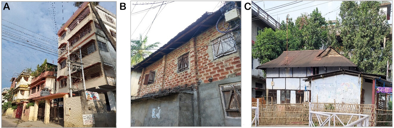
Figure 2. Observed MBTs (A) RC, (B) unreinforced masonry, and (C) Assam-type buildings at Silchar City.
Building parameters considered
| S.No. | Variables |
| 1. | Width of beam (WB) |
| 2. | Beam depth (BD) |
| 3. | Column width (CW) |
| 4. | Column depth (CD) |
| 5. | Concrete grade (fck) |
| 6. | Rebar grade (fy) |
| 7. | Bay width (BW) |
| 8. | Number of bays (NB) |
| 9. | Ground floor (GF) height |
| 10. | Other floors' (OF) height |
| 11. | Live load (LL) |
| 12. | Percentage of steel (PS) |
In practice, a collection of RC buildings typically consists of structures with varying heights, and each of these buildings will respond differently to earthquakes. To predict damage, a different response surface model is required for each individual building. However, in the case of Silchar City, only buildings up to 4 stories are available. Therefore, this study will focus only on 4-storey buildings, specifically the class of mid-rise concrete frame with unreinforced masonry infill walls (C3-M according to HAZUS building classification)[3]. The low-rise buildings are not chosen, as the substantial difference is not seen in the building properties between 4-storey buildings and those with fewer stories. The range of each variable, as shown in Table 3, is created by specifying the operating range of each input variable so that the range mostly encompasses the region where the probability density of the structural parameters is highest. The range of each variable is according to the observation from RVS data and expert opinions.
Observed lower bound and upper bound values of each input variable
| Variables | Range Value |
| WB | 250-350 (mm) |
| BD | 250-450 (mm) |
| CW | 250-450 (mm) |
| CD | 300-600 (mm) |
| fck | M15-M30 |
| fy | Fe250-Fe500 |
| BW | 3-6 (m) |
| NB | 3-8 |
| GF | 3.5-4.5 (m) |
| OF | 3-3.5 (m) |
| LL | 2-5 kN/m2 |
| PS | 1.5%-3% |
Screening of variables
The selected input variables must be tested to ensure that only the most significant input variables are taken into consideration when building the model while excluding other variables from further analysis. This increases the efficiency of the RSM. The Plackett-Burman screening design is used to construct a sample of various building cases, considering the variables mentioned in Table 2. The maximum inter-story drift values (in per cent), represented by the outputs (IDR), are calculated by performing NLTHA on each building model case. A first-order regression model has been generated with these output values to identify the most significant variables. The generated building cases, along with the outputs and the resulting regression equation, are discussed in the
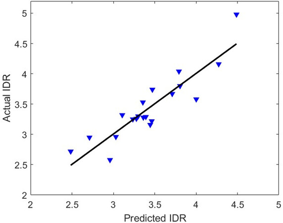
Figure 3. The plot of actual versus predicted IDR.
Statistical validation measures for the model.
| Statistical measure | Percentage (%) |
| R2 | 81 |
| (RA)2 | 78 |
| %AvgErr | 6.7 |
| %RMSE | 5.3 |
A screening design has been conducted, and based on Figure 4, it has been observed that among these 12 input variables, BW is the most significant variable, while NB has the least importance. In this study, the first seven parameters (BW, fck, LL, CD, BD, PS, and CW) are considered since they account for over 80% of the total response. As a result, only these seven parameters are considered as variables, and the remaining five parameters are assigned deterministic values.
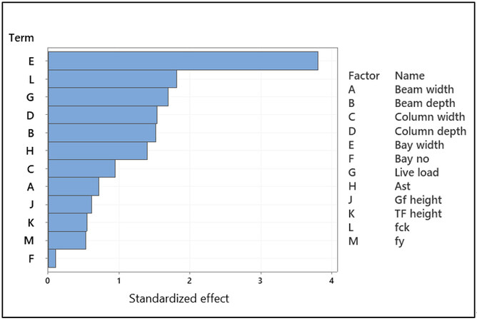
Figure 4. Significance of input variables.
Response surface model generation
As previously discussed, three codal design provisions are considered to account for the age of the building. The codal provision IS 1893:1984[34] is used to design buildings constructed between 1984 and 2002. Similarly, IS 1893:2002[35] and IS 1893:2016[36] are used to design buildings constructed between 2002 and 2016 and from 2016 to the present, respectively. Therefore, three response surface metamodels are developed. Table 5 shows the lower-upper bound values of the input variables according to the construction age of the building. Table 6 shows the deterministic values of the five parameters that are excluded after screening.
Lower bound and upper bound values as per age of the building
| Variables | HC | MC | LC |
| BD | 350-450 mm | 300-350 mm | 250-280 mm |
| CW | 400-450 mm | 300-400 mm | 250-300 mm |
| CD | 450-600 mm | 400-500 mm | 300-350 mm |
| BW | 3.5-6 m | 3.5-4.5 m | 3-3.5 m |
| fck | M20-M30 | M15-M25 | M15-M25 |
| LL | 2-5 kN/m2 | 2-5 kN/m2 | 2-5 kN/m2 |
| PS | 2%-3% | 1.5%-2.5% | 1.5%-2% |
Fixed values of the non-significant parameters
| Parameters | HC | MC | LC |
| WB | 300 | 300 | 250 |
| NB | 4 × 4 | 4 × 4 | 4 × 4 |
| GF | 4 m | 4 m | 4 m |
| OF | 3.2 m | 3.2 m | 3.2 m |
| fy | Fe 500 | Fe 415 | Fe 415 |
As previously mentioned, the PGA variable is also added to the existing set of seven variables, resulting in a total of eight variables (BD, CW, CD, BW, fck, LL, PS, and PGA). For each response surface metamodel, three sets of sampling points or building model cases are constructed using CCD with these eight variables. Each set consists of 81 building model cases, amounting to a total of 243 cases. NLTHA is carried out on all 243 building cases, with each building case subjected to 11 ground motions (as outlined in Table 1) scaled to either 0.1 g (lower bound), 0.35 g (centre bound), or 0.6 g (upper bound) based on the generated cases. Eleven IDRs are extracted for each case, and the mean and standard deviation of IDR is obtained as discussed. Second-order polynomial response functions or metamodels are generated for the mean (µ) and standard deviation (σ) of IDR using least square regression analysis for HC, MC, and LC and are shown in the
Where IDRHC is the overall response surface metamodel of a collection of buildings designed according to HC, IDRμHC represents the metamodel for the mean of the response, and N[0, IDRσHC] incorporates unpredictability in seismic excitations by representing the dispersion among earthquakes in response calculation. Table 7 lists the statistical validation of the regression models, and it has been observed that the level of error in the model is extremely low, indicating the prediction accuracy of the regression model. Figure 5 displays a plot of the actual IDR values obtained from the NLTHA compared to the values predicted by the regression model. The trendline represents a good fit between the actual and the predicted values.
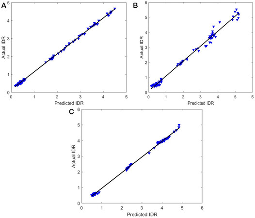
Figure 5. The plot of actual versus predicted IDR for (A) HC, (B) MC, and (C) LC.
Statistical validation measures for the models
| Statistical measure | HC (in %) | MC (in %) | LC (in %) |
| R2 | 98.79 | 98.7 | 99.78 |
| (RA)2 | 97.34 | 97.14 | 99.52 |
| %AvgErr | 7.66 | 8.33 | 3.18 |
| %RMSE | 7.29 | 6.36 | 2.55 |
Response simulation
MCS is now performed using the metamodel shown in Equation (6) to obtain various values of IDRs, replacing the need for time-consuming NLTHA. The Probability Density Function (PDF) is used to represent the distribution of input variables during MCS. Probability distributions of the input variables are defined as shown in Table 8, allowing for the simulation of different values of IDR. The units of variables are specified in Table 3. As the building inventory data is based on RVS data and expert opinions, it is difficult to identify the probability distribution of the input variables due to the unavailability of realistic statistical data. As a result, the mean values of the variables are assumed based on the values in Table 5, while the probability distributions of the variables and their measures of dispersion are gathered from previous investigations[64-67].
Input variables and their probability distribution parameters
| Variables | Distribution | HC | MC | LC | |||
| µ | σ | µ | σ | µ | σ | ||
| BD | Normal | 400 | 8 | 325 | 6.5 | 265 | 5.6 |
| CW | Normal | 425 | 63.75 | 350 | 52.5 | 275 | 22 |
| CD | Normal | 500 | 130 | 450 | 117 | 325 | 81.25 |
| BW | Uniform | 4.75 | 0.52 | 4 | 0.083 | 3.25 | 0.0208 |
| fck | Normal | 25 | 3.75 | 20 | 3 | 20 | 1.6 |
| LL | Lognormal | 3 | 1.56 | 3 | 1.56 | 3 | 1.56 |
| PS | Normal | 2.5 | 0.1 | 2 | 0.08 | 1.75 | 0.07 |
The Monte Carlo sampling is used to choose input variable values according to their probability distributions. Each simulation step combines these input variables to represent a building model case with corresponding properties. The IDR value is then obtained by evaluating both metamodels (IDRμHC and
As discussed, the metamodels are evaluated at specific intensity levels to determine the IDR value. For example, at PGA = 0.1 g, MCS is performed 10,000 times using Equation (6) by random selection of the values of input variables based on their assumed probability distribution [Table 8]. The IDR is obtained 10,000 times through this process. The exceeding probability of limit states (1% drift for IO, 1.5% drift for LS, and 2.5% drift for CP) is obtained by dividing the number of times the computed response exceeds the limit state thresholds by the total number of simulation trials (10,000 trials). This process is repeated till
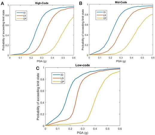
Figure 6. Fragility curves representing the overall damage level of the portfolio of buildings constructed during the year (A) 2016-present, (B) 2002-2016, and (C) 1984-2002.
Probability of exceeding values for three limit states (HC)
| PGA | IO | LS | CP |
| 0.1 g | 0.0278 | 0.0089 | 0.0026 |
| 0.2 g | 0.2331 | 0.0361 | 0.0038 |
| 0.3 g | 0.7444 | 0.2836 | 0.0139 |
| 0.4 g | 0.9174 | 0.7435 | 0.1191 |
| 0.5 g | 0.9537 | 0.9059 | 0.4566 |
| 0.6 g | 0.9649 | 0.9467 | 0.7754 |
RESULTS AND DISCUSSIONS
The fragility curves in Figure 6 present the overall damage levels of a collection of RC buildings in Silchar City. It is observed that the probability of exceeding 1%, 1.5%, and 2.5% drift is higher for buildings designed according to the lower version of code compared to those designed according to newer versions. It indicates the fact that older buildings are more vulnerable to damage due to strength degradation than newer ones. It is interesting to note how the construction age of the buildings plays a crucial role in the damage assessment. However, it is worth noting that according to FEMA, 2009[47] guidelines, the probability of failure of any individual building at the specified hazard level should be less than 20%. Silchar City, located in seismic Zone V in Northeast India, adopts the MCE hazard level of 0.36 g for HC and MC and 0.4 g for LC[34,36,37] in the design of the buildings. As the CP damage level corresponds to substantial damage and indicates a moment close to collapse, reaching the CP level drift is considered a failure. Therefore, Figure 6 demonstrates that none of the buildings in Silchar City shows a probability of failure corresponding to their respective hazard levels for which they were designed.
Each fragility curve corresponds to the three drift limit states for a particular design code provision: HC, MC, and LC. These curves show the damage levels for a collection of buildings. It is not possible to obtain the damage level for a specific building using the metamodel, as described in Equation (6). There is a need to modify the metamodel so that it can be applied on an individual basis. This is where the assessment of building-specific fragility curves using RSM comes into the picture. Unlike the conventional method of performing NLTHA on each building, RSM can now be used as a tool to derive the fragility curve for an individual building by performing a simulation on the modified metamodel.
The metamodel applicable to a specific building is obtained by using values of the variables specific to that building in Equation (6). Subsequently, MCS is performed following the same procedure as described earlier. Table 10 shows four specific buildings with their own geometric and material properties, all designed according to the same code (HC). The purpose is to observe the variation in the fragility curves among the buildings designed with the same code.
Characteristics of the buildings designed according to IS 1893:2016 (HC)
| Building name | BD | CW | CD | fck | BW | LL | PS |
| B1 | 450 | 450 | 550 | 20 | 3.5 | 3 | 2.5% |
| B2 | 400 | 400 | 500 | 30 | 5 | 2.3 | 3% |
| B3 | 450 | 450 | 550 | 30 | 6 | 2.5 | 2.5% |
| B4 | 350 | 400 | 450 | 20 | 5 | 3.5 | 3% |
It is evident from Figure 7 that although the beam, column sizes, and PS are the same for B1 and B3, the fragility curve differs for all the limit states due to variations in BW, fck, and LL. These variables are the most significant based on the screening design shown in Figure 4. A similar observation can be made for B2 and B3, as their fragility curves exhibit a high degree of similarity. This can be attributed to the fact that the relatively significant variables (BW, fck and LL) have almost identical values for these two buildings. Therefore, by referring to the existing fragility curve developed using RSM, it is possible to predict the fragility curve of any building if the relatively most significant parameters are the same for both buildings.
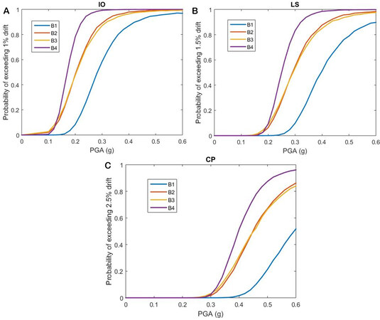
Figure 7. Fragility curve of buildings, (A) IO, (B) LS, and (C) CP limit states.
To validate this rapid method of obtaining the fragility curve, a thorough investigation is carried out on building B1 using traditional nonlinear time history studies. IDA has been performed to derive the fragility curve for building B1. The detailed analysis procedure of IDA can be found in[1,16,18]. Figure 8 shows the comparison of fragility curves derived using RSM and IDA. The resemblance of the fragility curves obtained using IDA with RSM validates the accuracy of the rapid fragility assessment using RSM.
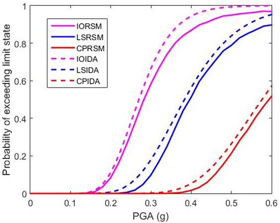
Figure 8. Comparison of RSM and IDA.
CONCLUDING REMARKS
With the aid of a simulation-based statistical method known as response surface metamodel, this study has considered building-to-building variability for determining the fragility of the portfolio of RC buildings in a region. The fragility curve indicates the probability of exceeding the damage state while considering uncertainty in both the building properties and earthquake forces. Although the uncertainty in earthquake forces is usually addressed by considering various ground motions, the complexity arises when building-to-building variability within a region needs to be considered. The computational efficiency reduces when the analysis needs to be done for every building located in a region. However, by incorporating building-to-building variability as input parameters within the existing RSM framework, the need for complex nonlinear analyses can be replaced with a more computationally efficient approach. The RSM establishes a relationship between the response of the building, the building input parameters, and ground motion intensity using simple polynomial functions or metamodels. A case study is performed on Silchar, a city in Northeast India, and several key findings of the study are as follows:
• The buildings in the city are classified according to their construction age, which is represented by different codal design provisions. This classification is done to take into account the strength degradation of RC buildings over time.
• Out of the 12 building input parameters considered, the width of the bay is found to be more significant, and the number of bays is less significant in the overall response (IDR) of the building.
• Using the metamodel developed, fragility curves are efficiently obtained, representing the damage level for a collection of buildings of three construction age classes of buildings.
• The old-aged buildings are found to be more vulnerable to damage, as the probability of exceeding the limit states for various seismic intensity levels is higher as compared to the newly constructed buildings.
• When examining the fragility of the four specific buildings, it is found that if the relatively significant building parameters (as obtained from screening design) are similar, the fragility curve shows similarities, even if the non-significant parameters vary.
• The RSM approach is validated against the conventional method, such as IDA, and it is found that both approaches show similar results, indicating the accuracy of rapid fragility assessment using RSM.
However, this methodology does have a limitation. The metamodel developed with this approach is applicable for a certain building class based on its height. The same metamodel cannot be applied to low-rise or high-rise structures. This shortcoming can be overcome by accommodating the building height as a variable, along with other building input parameters. However, the DoE techniques do not allow for the inclusion of building height as a variable. It is because when generating sampling points or building model cases using DoE, it does not account for the fact that high-storey buildings generally have a different range of values of input parameters compared to low-rise structures. Further investigation is needed to be done to overcome this limitation.
DECLARATIONS
AcknowledgementsThe authors highly acknowledge the reviewers for their valuable comments that have enhanced the quality of the manuscript. The first author (GR) acknowledges the students’ scholarship received from the Ministry of Human Resource and Development, Government of India.
Authors’ contributionsConceptualisation, methodology, software, investigation, writing: Roy G
Methodology, supervision, review, and editing: Dutta S, Choudhury S
Availability of data and materialsSome of the significant data are available with the corresponding author on request.
Financial support and sponsorshipNone.
Conflicts of interestAll authors declared that there are no conflicts of interest.
Ethical approval and consent to participateNot applicable.
Consent for publicationNot applicable.
Copyright© The Author(s) 2023.
REFERENCES
1. Roy G, Choudhury S, Dutta S. An integral approach to probabilistic seismic hazard analysis and fragility assessment for reinforced concrete frame buildings. J Perform Constr Facil 2021;35:04021097.
2. Towashiraporn P, Dueñas-Osorio L, Craig JI, Goodno BJ. An application of the response surface metamodel in building seismic fragility estimation. The Proceedings of the 14th World Conference on Earthquake Engineering, 12-17 October 2008; China. Available from: chrome-extension://efaidnbmnnnibpcajpcglclefindmkaj/https://www.fema.gov/sites/default/files/2020-09/fema_hazus_earthquake-model_technical-manual_2.1.pdf [Last accessed on 30 May 2023].
3. Federal Emergency Management Agency (FEMA). HAZUS technical and user’s manual of advanced engineering building module (AEBM) “Hazus MH 2.1” 2013.
4. Steneker P, Wiebe L, Filiatrault A, Konstantinidis D. A framework for the rapid assessment of seismic upgrade viability using performance-based earthquake engineering. Earthq Spectra 2022;38:1761-87.
5. Zareian F, Krawinkler H. Assessment of probability of collapse and design for collapse safety. Earthq Eng Struct Dyn 2007;36:1901-14.
6. Rizzano G, Tolone I. Seismic assessment of existing RC frames: probabilistic approach. J Struct Eng 2009;135:836-52.
7. Burton H, Deierlein G. Simulation of seismic collapse in nonductile reinforced concrete frame buildings with masonry infills. J Struct Eng 2014;140:A4014016.
8. Pujari NN, Ghosh S, Lala S. Bayesian approach for the seismic fragility estimation of a containment shell based on the formation of through-wall cracks. Am Soc Civil Eng 2016;2:B4015004.
9. Feng D, Sun X, Li Y, Wu G. Two-parameter-based damage measure for probabilistic seismic analysis of concrete structures. Am Soc Civil Eng 2023;9:04022061.
10. Kazemi F, Jankowski R. Seismic performance evaluation of steel buckling-restrained braced frames including SMA materials. J Constr Steel Res 2023;201:107750.
11. Prasad JS, Singh Y, Kaynia AM, Lindholm C. Socioeconomic clustering in seismic risk assessment of urban housing stock. Earthq Spectra 2009;25:619-41.
12. Surana M, Meslem A, Singh Y, Lang DH. Analytical evaluation of damage probability matrices for hill-side RC buildings using different seismic intensity measures. Eng Struct 2020;207:110254.
13. Kappos AJ, Panagopoulos G, Panagiotopoulos C, Penelis G. A hybrid method for the vulnerability assessment of R/C and URM buildings. Bull Earthq Eng 2006;4:391-413.
14. Haldar P, Singh Y. Seismic performance and vulnerability of indian code-designed RC frame buildings. ISET J Earthq Technol 2009;46:29-45.
15. Haselton CB, Baker JW, Liel AB, Deierlein GG. Accounting for ground-motion spectral shape characteristics in structural collapse assessment through an adjustment for epsilon. J Struct Eng 2011;137:332-44.
16. Baker JW. Efficient Analytical fragility function fitting using dynamic structural analysis. Earthq Spectra 2015;31:579-99.
17. Rodríguez J, Aldabagh S, Alam MS. Incremental dynamic analysis-based procedure for the development of loading protocols. J Bridge Eng 2021;26:04021080.
19. D’Ayala D, Meslem A, Vamvatsikos D, Porter K, Rossetto T, Silva V. Guidelines for analytical vulnerability assessment of low/mid-rise buildings. vulnerability global component project. GEM Technical Report 2015-08 v1.0.0 08:162. Available from: chrome-extension://efaidnbmnnnibpcajpcglclefindmkaj/https://cloud-storage.globalquakemodel.org/public/wix-new-website/pdf-collections-wix/publications/Guidelines%20for%20Analytical%20Vulnerability%20Assessment%20-%20Low_Mid-Rise.pdf [Last accessed on 30 May 2023].
20. Rajkumari S, Thakkar K, Goyal H. Fragility analysis of structures subjected to seismic excitation: a state-of-the-art review. Structures 2022;40:303-16.
21. Masoomi H, van de Lindt JW. Community-resilience-based design of the built environment. Am Soc Civil Eng 2019;5:04018044.
22. Gentile R, Galasso C. Gaussian process regression for seismic fragility assessment of building portfolios. Struct Saf 2020;87:101980.
23. Sousa R, Batalha N, Silva V, Rodrigues H. Seismic fragility functions for Portuguese RC precast buildings. Bull Earthq Eng 2021;19:6573-90.
24. Yoshikawa H, Goda K. Financial seismic risk analysis of building portfolios. Nat Hazards Rev 2014;15:112-20.
25. Lin P, Wang N. Building portfolio fragility functions to support scalable community resilience assessment. Sustain Resilient Infrastruct 2016;1:108-22.
26. Maio R, Tsionis G, Sousa ML, Dimova SL. Review of fragility curves for seismic risk assessment of buildings in Europe. The Proceedings of 16th World Conference on Earthquake Engineering; 9-13 January 2017; Santiago Chile.
27. Giordano N, De Luca F, Sextos A. Analytical fragility curves for masonry school building portfolios in Nepal. Bull Earthq Eng 2021;19:1121-50.
28. Martins L, Silva V. Development of a fragility and vulnerability model for global seismic risk analyses. Bull Earthq Eng 2021;19:6719-45.
29. Surana M, Singh Y, Lang DH. Seismic characterization and vulnerability of building stock in hilly regions. Nat Hazards Rev 2018;19:04017024.
30. Meneses-loja J, Aguilar Z. Seismic vulnerability of school buildings in Lima, Peru. The Proceedings of 13th World Conference on Earthquake Engineering, 1-6 August 2004; Vancouver, Canada.
31. Sarkar PK, Ghosh S, Chakraborty S. An efficient responses surface method for seismic fragility analysis of existing building frame. The Proceedings of 15th Symposium of Earthquake Engineering, October 2015; Roorkee.
32. Baker JW. Measuring bias in structural response caused by ground motion scaling. The Proceedings of 8th Pacific Conference on Earthquake Engineering, 5-7 December 2007; Singapore.
33. Gunthal G, Musson R, Schwarz J, Stucchi M. The European macroseismic scale (MSK-92). Terra Nova 1993;5:305-305. Available from: chrome-extension://efaidnbmnnnibpcajpcglclefindmkaj/https://law.resource.org/pub/in/bis/S03/is.1893.1984.pdf [Last accessed on 30 May 2023].
34. Indian standard criteria for earthquake resistant design of structures. New Delhi: Bureau of Indian Standards; 1893.
35. Bureau of Indian Standards New Delhi. Criteria for earthquake resistant design of structures - general provisions and buildings part-1. New Delhi: Bureau of Indian Standards; 2002; pp. 1-39.
36. Part-1. Criteria for earthquake resistant design of structures, Part 1: general provisions and buildings. New Delhi: Bureau of Indian Standards; 1893; pp. 1-44.
37. Antony J. Training for design of experiments using a catapult. Qual Reliab Eng Int 2002;18:29-35.
38. Antony J. Screening designs. Design of experiments for engineers and scientists. Amsterdam, The Netherlands: Elsevier; 2014. pp. 51-62.
39. Jones B, Nachtsheim CJ. Effective design-based model selection for definitive screening designs. Technometrics 2017;59:319-29.
40. Montgomery DC. Design and analysis of experiments, 8th edition. Hoboken, New Jersey: Wiley, 2013.
41. Simpson TW, Lin DKJ, Chen W. Sampling strategies for computer experiments: design and analysis. Int J Reliab Appl 2001;2:209-40. Available from: chrome-extension://efaidnbmnnnibpcajpcglclefindmkaj/http://www.personal.psu.edu/users/j/x/jxz203/lin/Lin_pub/2001_IJRA.pdf [Last accessed on 30 May 2023].
42. Lallemant D, Kiremidjian A, Burton H. Statistical procedures for developing earthquake damage fragility curves. Earthq Eng Struct Dyn 2015;44:1373-89.
43. Ader T, Grant DN, Free M, Villani M, Lopez J, Spence R. An unbiased estimation of empirical lognormal fragility functions with uncertainties on the ground motion intensity measure. J Earthq Eng 2020;24:1115-33.
44. Acevedo AB, Yepes-estrada C, González D, et al. Seismic risk assessment for the residential buildings of the major three cities in Colombia: Bogotá, Medellín, and Cali. Earthq Spectra 2020;36:298-320.
45. Tafti M, Amini Hosseini K, Mansouri B. Generation of new fragility curves for common types of buildings in Iran. Bull Earthq Eng 2020;18:3079-99.
46. Wen YK, Wu CL. Uniform hazard ground motions for mid-america cities. Earthq Spectra 2001;17:359.
47. FEMA P695. Quantification of building seismic performance factors. 2009; p. 421. Available from: chrome-extension://efaidnbmnnnibpcajpcglclefindmkaj/https://www.fema.gov/sites/default/files/2020-08/fema_earthquakes_quantification-of-building-seismic-performance-factors-component-equivalency-methodology-fema-p-795.pdf [Last accessed on 30 May 2023].
48. Americal society of civil engineers (ASCE/SEI 7-16). Minimum design loads and associated criteria for buildings and other structures. 2017.
49. Roy G, Choudhury S, Dutta S. A Case study of probabilistic seismic hazard analysis using grid-based approach in area sources and computation of hazard deaggregation. In: Fonseca de Oliveira Correia JA, Choudhury S, Dutta S, editors. Advances in structural mechanics and applications. Cham: Springer International Publishing; 2022. pp. 479-93.
50. Roy G, Dutta S, Choudhury S. An integrated uncertainty quantification framework for probabilistic seismic hazard analysis. Am Soc Civil Eng 2023;9:04023017.
51. Rodriguez ME, Aristizabal JC. Evaluation of a seismic damage parameter. Earthq Eng Struct Dyn 1999;28:463-77.
52. Wong KKF, Wang Y. Energy-based damage assessment on structures during earthquakes. Struct Des Tall Build 2001; 10:135-54.
53. Park Y, Ang AH, Wen YK. Seismic damage analysis of reinforced concrete buildings. J Struct Eng 1985;111:740-57.
54. Mibang D, Choudhury S. Damage index evaluation of frame-shear wall building considering multiple demand parameters. J Build Rehabil 2021;6:40.
55. Mibang D, Choudhury S. Prediction evaluation of Global damage index of RC dual system buildings by support vector regression method. Innov Infrastruct Solut 2022;7:169.
56. ASCE. Fema 356. Prestandard and commentary for the seismic rehabilitation of building. Rehabilitation 2000. Available from: chrome-extension://efaidnbmnnnibpcajpcglclefindmkaj/https://www.nehrp.gov/pdf/fema356.pdf [Last accessed on 30 May 2023].
57. Kircher CA. Earthquake loss estimation methods for welded steel moment-frame buildings. Earthq Spectra 2003;19:365-84.
59. Papila M, Haftka RT. Response surface approximations: noise, error repair, and modeling errors. AIAA J 2000;38:2336-43.
60. FEMA 274, ATC, NEHRP commentary on the guidelines for the seismic rehabilitation of buildings. Washington, DC: Federal Emergency Management Agency; 1997.
61. Choudhury S, Singh SM. A unified approach to performance-based design of RC frame buildings. J Inst Eng India Ser A 2013;94:73-82.
62. Das TK, Choudhury S. Developments in the unified performance-based seismic design. J Build Rehabil 2023;8:13.
63. Kayal JR. Seismotectonics of Northeast India: a review. J Geophys 1998;19:9-34. Available from: https://www.semanticscholar.org/paper/Seismicity-of-northeast-India-and-surroundings-%3A-Kayal/e3a47c0ab06918f78a8a9da5d7672023c33ff826 [Last accessed on 30 May 2023].
64. Srividya A, Ranganathan R. Reliability based optimal design of reinforced concrete frames. Comput Struct 1995;57:651-61.
65. Lu R, Luo Y, Conte JP. Reliability evaluation of reinforced concrete beams. Struct Saf 1994;14:277-98.
66. Ozmen HB, Inel M, Senel SM, Kayhan AH. Load carrying system characteristics of existing Turkish RC building stock. Int J Civil Eng 2015;13:76-91.
Cite This Article
Export citation file: BibTeX | RIS
OAE Style
Roy G, Dutta S, Choudhury S. Building portfolio seismic fragility analysis: incorporating building-to-building variability to carry out seismic fragility analysis for reinforced concrete buildings in a city. Dis Prev Res 2023;2:6. http://dx.doi.org/10.20517/dpr.2023.08
AMA Style
Roy G, Dutta S, Choudhury S. Building portfolio seismic fragility analysis: incorporating building-to-building variability to carry out seismic fragility analysis for reinforced concrete buildings in a city. Disaster Prevention and Resilience. 2023; 2(2): 6. http://dx.doi.org/10.20517/dpr.2023.08
Chicago/Turabian Style
Roy, Geetopriyo, Subhrajit Dutta, Satyabrata Choudhury. 2023. "Building portfolio seismic fragility analysis: incorporating building-to-building variability to carry out seismic fragility analysis for reinforced concrete buildings in a city" Disaster Prevention and Resilience. 2, no.2: 6. http://dx.doi.org/10.20517/dpr.2023.08
ACS Style
Roy, G.; Dutta S.; Choudhury S. Building portfolio seismic fragility analysis: incorporating building-to-building variability to carry out seismic fragility analysis for reinforced concrete buildings in a city. Dis. Prev. Res. 2023, 2, 6. http://dx.doi.org/10.20517/dpr.2023.08
About This Article
Copyright

Data & Comments
Data


 Cite This Article 19 clicks

 Like This Article 1
likes
Like This Article 1
likes


Comments
Comments must be written in English. Spam, offensive content, impersonation, and private information will not be permitted. If any comment is reported and identified as inappropriate content by OAE staff, the comment will be removed without notice. If you have any queries or need any help, please contact us at support@oaepublish.com.